ChronoEarth-492K

Abstract

Hyperspectral imaging (HSI) provides dense spectral information for the Earth's surface, enabling material-level understanding of land cover and ecosystem dynamics. Despite recent progress in hyperspectral self-supervised learning (SSL), existing datasets remain temporally shallow, limiting the development of long-horizon spatiotemporal modeling. To address this gap, we introduce ChronoEarth-492K, the first large-scale, temporally calibrated hyperspectral SSL dataset built upon NASA's EO-1 Hyperion mission — the world's longest continuous hyperspectral archive (2001–2017). ChronoEarth-492K comprises 492,354 radiometrically harmonized patches across 185,398 global locations over 17 years, with 28,786 sites containing multi-temporal sequences (≥3 observations) that enable both short- and long-horizon temporal analysis. Building on this foundation, we establish the ChronoEarth-Benchmark, a unified evaluation suite spanning static, short-horizon, and long-horizon temporal tasks, constructed from six open-source geospatial products covering land cover, crop type, forest dynamics, and soil properties. We further introduce a standardized evaluation protocol and report extensive baseline results across state-of-the-art hyperspectral foundation models.

Key Contributions

1
ChronoEarth-492K dataset — the first large-scale hyperspectral SSL dataset offering 17 years of temporally calibrated global observations from NASA EO-1 Hyperion (2001–2017), with 492,354 patches at 30 m resolution across 9 global regions.
2
ChronoEarth-Benchmark — a unified evaluation suite with static, short-horizon, and long-horizon temporal tasks across six geospatial products, with leak-proof spatial splits designed for realistic OOD evaluation.
3
Extensive baselines — comprehensive empirical evaluation of state-of-the-art hyperspectral foundation models (SpectralViT, LESSViT, DOFA, HyperSigma, SatMAE, DINOv3) under static, temporal, and cross-satellite transfer settings.

Data Collection & Processing Pipeline

ChronoEarth-492K is built from the complete NASA EO-1 Hyperion Level-1T archive (May 2001 – March 2017), the longest-running spaceborne hyperspectral mission to date. The pipeline consists of four stages:

🛰️

1. Data Acquisition

All Level-1T terrain-corrected Hyperion scenes with <10% cloud cover are queried from the USGS EROS archive via the M2M API. Nine continental regions are defined to ensure geographic balance and limit oceanic coverage.

🌈

2. Spectral Harmonization

Each scene contains 242 raw bands. Following established protocols, unstable and low-signal bands (water absorption at ~1400 nm and ~1900 nm, instrument noise bands) are removed, retaining 155 spectrally consistent bands across all scenes.

🗺️

3. Global Patching & Indexing

Scenes are resampled to 30 m and divided into non-overlapping 128×128 pixel patches aligned to a fixed UTM-zone global grid. Each patch receives a deterministic UID encoding its UTM zone, column, and row, enabling consistent cross-timestamp alignment.

⏱️

4. Temporal Sequence Construction

Patches sharing the same UID but different timestamps are grouped into spatiotemporal sequences. This yields 56,491 locations with ≥2 observations and 28,786 locations with ≥3 timestamps, supporting both short- and long-horizon modeling.

Global patching and spatiotemporal indexing pipeline

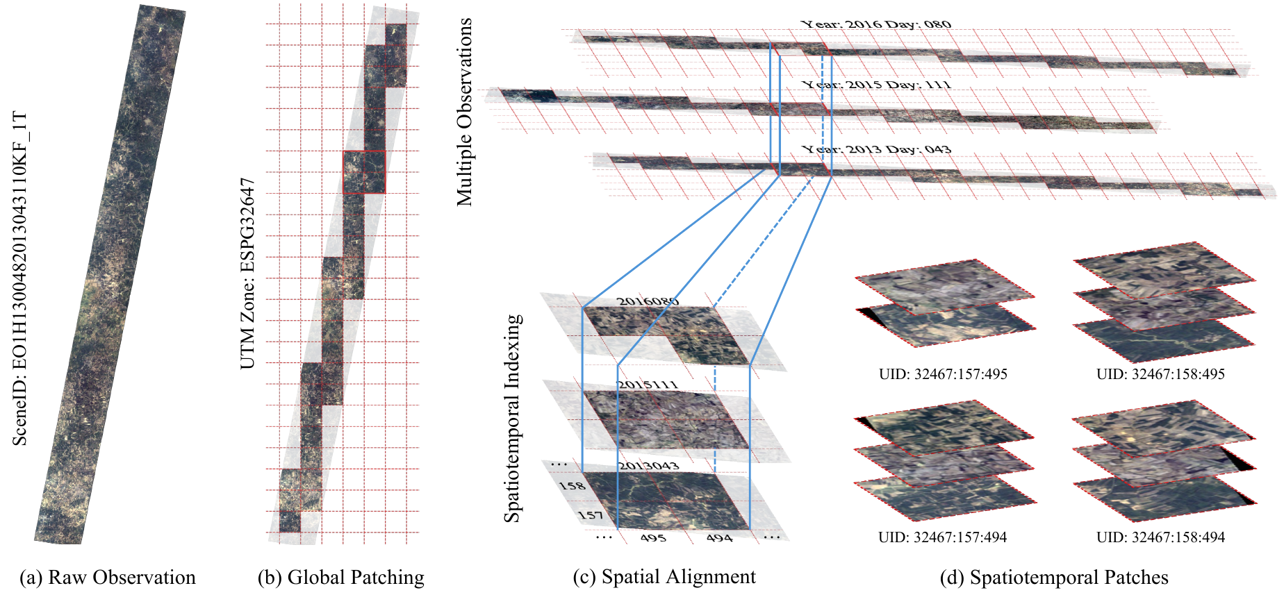
Figure: Global Patching and Spatial Alignment. (a) Raw EO-1 Hyperion observation. (b) Global patching using a UTM-zone–specific grid, with each patch assigned a unique spatial UID. (c) Spatial alignment of patches sharing the same UID across multiple observations. (d) Formation of spatiotemporal sequences by aggregating aligned samples from different timestamps.

Benchmark Label Processing

To construct the ChronoEarth-Benchmark, we align six geospatial label products with the hyperspectral imagery using the UID-based spatial index. Each label layer is projected to the corresponding UTM grid, and all valid location–label pairs are retained as supervision targets — enabling multi-year temporal task construction. Two quality filters are applied:

Class filtering: Labels with frequency below 1% are grouped into a background class to reduce noise from rare categories.
Entropy filtering: Patches with normalized Shannon entropy below τ = 0.1 are discarded, retaining only semantically informative samples.

Leak-proof train/val/test splits are generated by a distance-aware grouping strategy based on EO-1 orbital swaths. Patches from the same acquisition are grouped into spatial units, and overlapping units are merged into connected components. Splits are assigned at the component level, inducing a spatial OOD setting where test samples come from geographically distinct regions.

Dataset Statistics

492K

Total patches

185K

Unique locations

28.8K

Multi-temporal sites (≥3 obs.)

17 yrs

Temporal span (2001–2017)

155

Spectral bands

30 m

Spatial resolution

Global regions

128²

Patch size (pixels)

Global Coverage

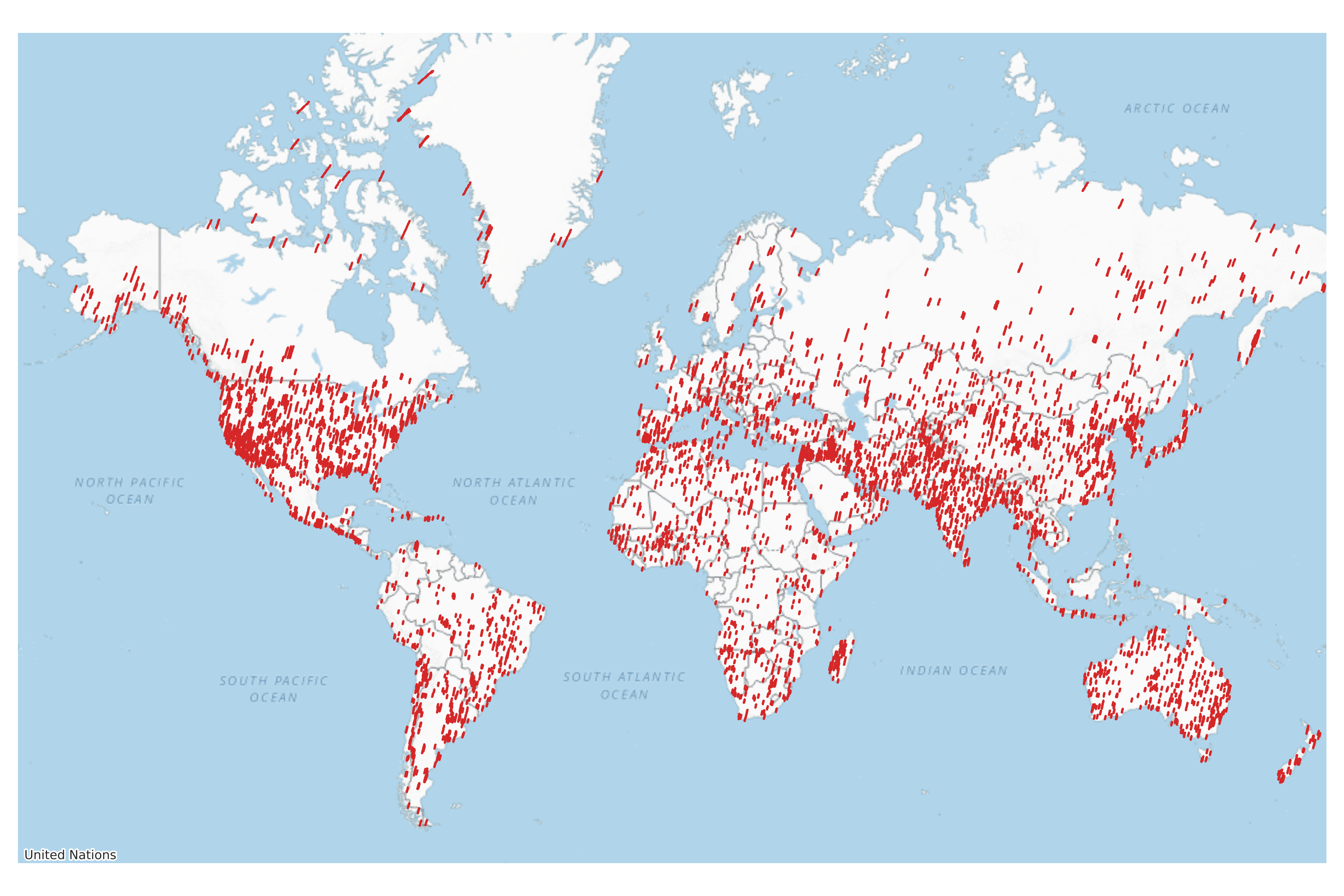
Figure: Global spatial coverage of ChronoEarth-492K. Red markers indicate hyperspectral observation locations distributed across Africa (AF), Arctic (AC), East Asia (EA), Europe (EU), Latin America (LA), North America (NA), Oceania (OC), Southeast Asia (SEA), and Southwest Asia (SWA).

Temporal Distribution

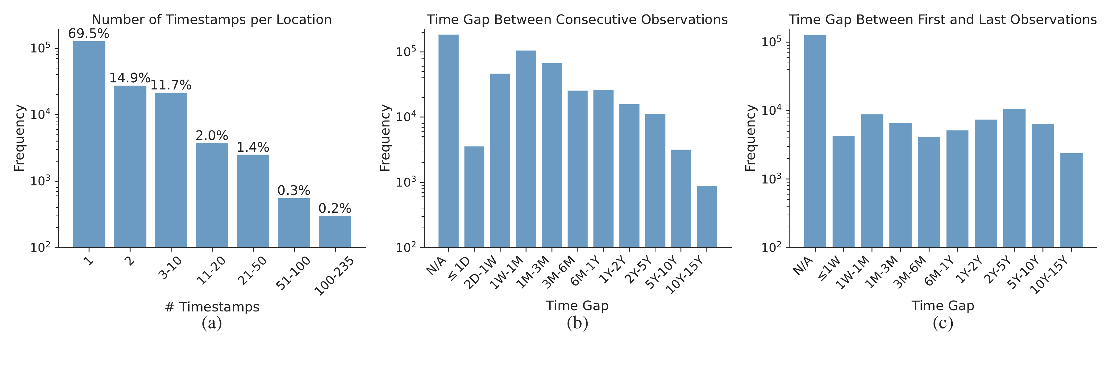
Figure: Temporal distribution of ChronoEarth-492K. (a) 69.5% of locations have a single observation; 28,786 locations have ≥3 timestamps enabling long-horizon modeling. (b) Time gaps between consecutive acquisitions are broadly distributed, from days to years. (c) Temporal coverage span per location — over one-third of multi-temporal sites span more than 2 years.

Spectral Groups

Group	Band IDs	Wavelength Range	# Channels
VNIR	B010 – B057	447 – 925 nm	48
SWIR1	B081 – B097	952 – 1114 nm	17
SWIR2	B101 – B119	1154 – 1336 nm	19
SWIR3	B134 – B164	1487 – 1790 nm	31
SWIR4	B182 – B221	1971 – 2365 nm	40
All		447 – 2365 nm	155

Comparison with Existing Hyperspectral SSL Datasets

Dataset	# Images	Patch Size	Sensor	Bands	GSD	Temporal Coverage
HySpecNet-11k	~11k	128×128	EnMAP	202	30 m	✗
MSST	~20k	64×64	EnMAP	200	30 m	✗
HSIHybrid	~4M	9×9	Multiple	Var.	—	✗
HyperGlobal-450K	~447k	64×64	EO-1 & GF-5B	242/330	30 m	✗
SpectralEarth	~538k	128×128	EnMAP	202	30 m	2 Years
ChronoEarth-492K ours	~492k	128×128	EO-1	155	30 m	17 Years

ChronoEarth-Benchmark

ChronoEarth-Benchmark integrates six open-source geospatial annotation products, covering land cover, crop type, forest dynamics, and soil properties across multiple continents. Three task types are defined:

Static

Single hyperspectral observation paired with the same-year label. Segmentation and multi-label classification.

Short-Horizon (SH)

Multiple temporally adjacent observations for the same label (T ≤ 4). Models aggregate short-term context under full supervision.

Long-Horizon (LH)

Future prediction: observations from 2001 to year n predict labels at year n+1. Tests temporal forecasting under partial supervision.

Dataset	Region	Classes	Task Type	Static samples	SH samples	LH samples
GFC	Global	1	Forest Change Detection	5,509	—	—
ISDASoil	Africa	8	Soil Classification	17,808	1,549	—
CDL	USA	12	Crop Type Segmentation	10,162	1,762	538
CORINE	Europe	19	Land Cover Classification	19,774	—	—
NLCD-S	USA	16	Land Cover Segmentation	55,476	4,077	1,812
CLCD	China	7	Land Cover Segmentation	17,614	1,069	460

Benchmark Dataset Illustrations

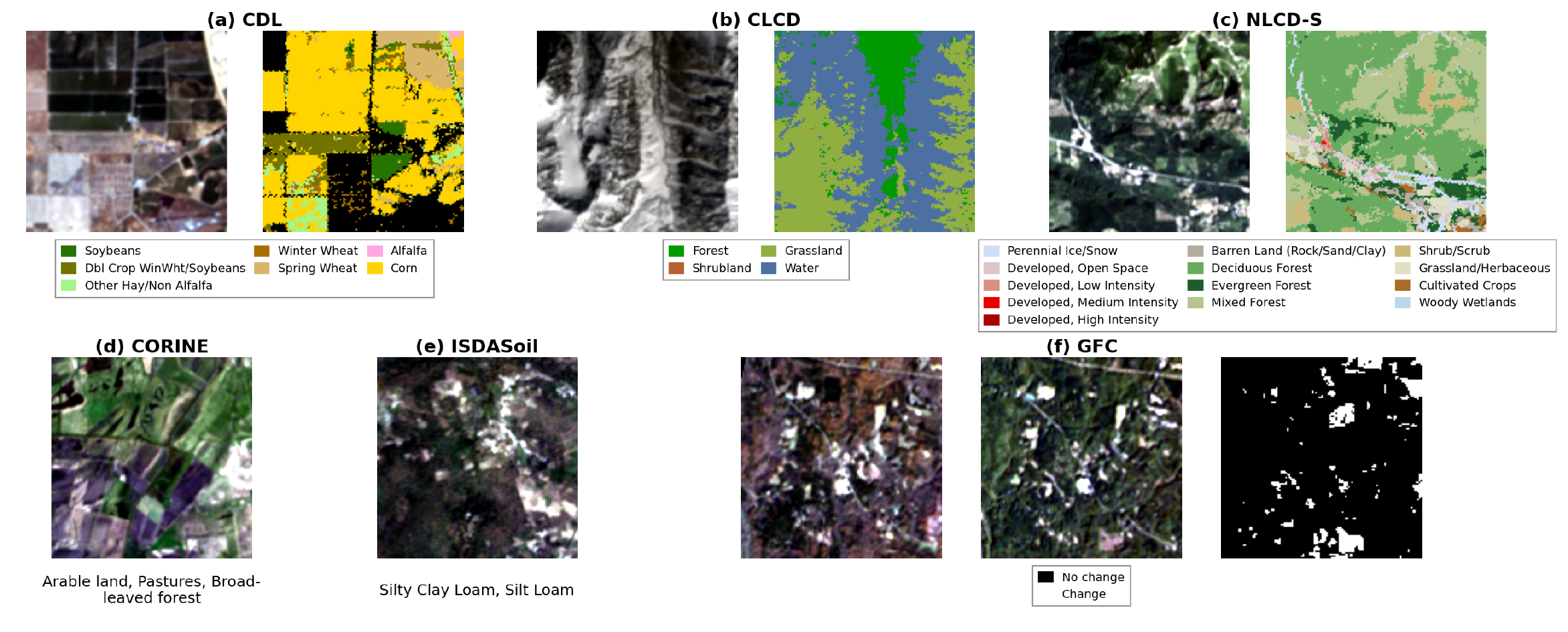
Sample patches from each benchmark dataset

Figure: Example patches from the six benchmark datasets. (a) CDL crop type with soybean, wheat, and corn labels. (b) CLCD Chinese land cover including forest, grassland, and shrubland. (c) NLCD-S US land cover across 16 classes. (d) CORINE European land cover. (e) ISDASoil Africa soil texture classification. (f) GFC forest change detection (black = no change, white = change).

Generalization Settings

Spatial-Temporal Generalization (CORINE). Data is split into temporal ID (2001–2012) and temporal OOD (2013–2017), then further divided by distance-aware spatial grouping. This yields four evaluation conditions: in-distribution (ID), temporal OOD (T-OOD), spatial OOD (S-OOD), and joint spatial-temporal OOD (ST-OOD).

Continental Generalization (GFC). Models are trained on data-rich regions (Europe, North America, East Asia) and evaluated on underrepresented continents (Africa, Latin America, Oceania, Southwest Asia), simulating real-world annotation imbalance.

Benchmark Results

We evaluate six hyperspectral foundation models: SpectralViT, LESSViT, DOFA, HyperSigma, SatMAE, and DINOv3 (adapted), all at ViT-Base scale. Sup. denotes supervised training from random initialization without self-supervised pretraining. Bold = best per column; italic red ↓ = performance degrades when more frames are added.

Static Tasks

Static Task Results

Self-supervised pretraining on ChronoEarth consistently improves over supervised counterparts. LESSViT achieves the best overall performance, demonstrating the benefit of architectures that explicitly model spatial–spectral interactions.

Method	CLCD mIoU ↑	CDL mIoU ↑	NLCD-S mIoU ↑	ISDASoil mAP ↑
DOFA	47.77	12.60	24.08	51.20
HyperSigma	41.53	11.45	23.05	54.50
DINOv3	47.10	11.65	24.46	50.90
SatMAE	41.25	11.94	22.23	49.80
ChronoEarth Pretrained
Sup. SpectralViT	48.01	15.50	29.10	57.79
SpectralViT	53.29	20.87	30.80	57.70
Sup. LESSViT	37.66	3.49	19.05	50.15
LESSViT	54.84	23.91	33.59	56.02

Generalization

CORINE: Spatial-Temporal Generalization (mAP ↑)

Performance degrades progressively from ID → T-OOD → S-OOD → ST-OOD, with spatial shift introducing the largest drop. SpectralViT and LESSViT pretrained on ChronoEarth achieve the highest scores across all OOD settings.

Method	ID	T-OOD	S-OOD	ST-OOD
DOFA	70.08	62.77	57.85	51.80
HyperSigma	59.99	58.09	54.75	49.18
DINOv3	58.93	54.88	50.80	46.00
SatMAE	67.26	58.69	55.77	47.20
ChronoEarth Pretrained
Sup. SpectralViT	74.14	63.30	60.48	55.21
SpectralViT	83.98	68.52	64.15	56.19
Sup. LESSViT	55.47	51.34	49.01	47.20
LESSViT	84.07	68.22	62.52	58.56

GFC: Cross-Continental Generalization

All methods degrade from ID to OOD, reflecting the difficulty of cross-continental transfer under annotation imbalance. SpectralViT outperforms LESSViT in this sparse-supervision setting, where strong spatial aggregation matters more than fine-grained spectral modeling.

Method	ID		OOD (Cross-Continental)
	mIoU ↑	F1 ↑	mIoU ↑	F1 ↑
DOFA	16.99	29.05	12.77	22.65
DINOv3	15.91	27.45	11.51	20.64
SatMAE	9.56	17.45	2.96	5.74
ChronoEarth Pretrained
Sup. SpectralViT	23.26	37.74	16.04	27.65
SpectralViT	29.90	46.04	19.38	32.47
Sup. LESSViT	0.00	0.00	0.00	0.00
LESSViT	19.29	32.34	16.13	27.78

Cross-Satellite Transfer

Cross-Satellite Generalization (SpectralViT backbone)

Models pretrained on ChronoEarth (EO-1 Hyperion) are fine-tuned and evaluated on EnMAP-based downstream tasks from SpectralEarth. Despite originating from a different and decommissioned sensor, ChronoEarth representations match or exceed those trained on in-domain EnMAP data.

Pretraining Data	BDFORET mIoU ↑	BNETD mIoU ↑	EuroCrops mIoU ↑	CORINE mAP ↑	CDL mIoU ↑
SpectralEarth (EnMAP)	76.30	49.46	69.34	75.33	77.44
ChronoEarth (ours)	76.39	44.34	69.82	79.02	73.66

Temporal Tasks

Short-Horizon Tasks (mIoU / mAP ↑)

Comparing T=1 (static) vs. T≤4 (multi-frame). Adding temporal context generally improves performance. The temporally pretrained SpectralViT consistently outperforms max-pooling and supervised attention aggregation, demonstrating the value of temporal SSL.

Method	CLCD (mIoU ↑)		CDL (mIoU ↑)		NLCD-S (mIoU ↑)		ISDASoil (mAP ↑)
	T=1	T≤4	T=1	T≤4	T=1	T≤4	T=1	T≤4
DOFA _max	39.88	39.76 ↓	12.68	14.88	14.96	18.25	52.80	50.63 ↓
DINOv3 _max	40.39	39.27 ↓	10.80	13.51	11.07	16.98	47.32	48.89
SatMAE _max	34.88	37.78	12.34	12.41	15.14	16.83	49.53	50.99
LESSViT _max	51.19	54.69	24.80	26.15	30.58	31.02	57.33	58.04
SpectralViT variants (ChronoEarth pretrained)
SpectralViT _max	43.37	44.55	16.47	20.07	19.90	19.82 ↓	56.49	56.72
SpectralViT _attention	—	43.77	—	18.97	—	22.88	—	48.98
SpectralViT _{temporal SSL}	—	45.57	—	22.64	—	23.59	—	54.14

Long-Horizon Tasks (mIoU ↑)

Evaluating future state prediction under increasing temporal history (T≤2, T≤4, T≤8). Longer history generally helps for CLCD and NLCD-S (gradual land-cover change), while CDL (crop type) shows less stable gains — longer history may introduce outdated or noisy signals for time-sensitive targets. Temporal SSL pretraining provides consistent gains.

Method	CLCD (mIoU ↑)			NLCD-S (mIoU ↑)			CDL (mIoU ↑)
	T≤2	T≤4	T≤8	T≤2	T≤4	T≤8	T≤2	T≤4	T≤8
DOFA _max	25.51	35.34	38.97	18.76	19.51	22.64	6.02	10.27	10.44
DINOv3 _max	20.26	33.72	37.04	18.14	20.34	21.83	5.25	9.35	11.22
SatMAE _max	20.00	31.25	29.85 ↓	13.66	18.22	19.40	5.43	10.19	11.80
LESSViT _max	38.80	50.08	54.64	28.36	33.75	35.52	9.97	18.83	14.43 ↓
SpectralViT variants (ChronoEarth pretrained)
SpectralViT _max	35.88	40.70	49.25	25.67	28.44	30.11	11.95	13.60	11.37 ↓
SpectralViT _attention	24.28	32.63	37.75	25.31	26.97	27.37	7.43	7.12 ↓	4.53 ↓
SpectralViT _{temporal SSL}	43.61	51.26	55.61	37.34	39.69	40.76	5.92	10.35	9.55 ↓

Citation

If you find ChronoEarth-492K useful in your research, please cite our paper:

@misc{si2026chronoearth492klargescalelong, title={ChronoEarth-492K: A Large Scale and Long Horizon Spatiotemporal Hyperspectral Earth Observation Dataset and Benchmark}, author={Haozhe Si and Yuxuan Wan and Yuqing Wang and Minh Do and Han Zhao}, year={2026}, eprint={2605.15666}, archivePrefix={arXiv}, primaryClass={cs.CV}, url={https://arxiv.org/abs/2605.15666}, }

arXiv

Dataset Code